Policy Center for the New South – Research Paper RP 02-23

Emran Sabrine[1] and Canuto Otaviano[2]

Abstract

This paper explores the impact of commodities financialization on crude oil prices and their volatility.  While some commodities have been market movers for centuries, introducing others, such as oil, to the financial markets is more recent. The increase in investors’ appetite for commodity investing has led to commodities’ financialization, which is often considered an amplifier of commodity price volatility. This paper focuses on the relationship between crude oil prices and the financialization argument through the commitment of traders undertaking long and short positions on the WTI crude oil to study their impact on spot prices and, thus, on crude oil’s volatility.

It reviews recent swings in oil prices and the correlation between prices of crude oil and speculative positions in financial markets. It also focuses on the relationship between crude oil prices, speculative positions, and volatility represented by the CBOE Crude Oil Volatility ETF through econometric models.

The aim is to bring additional information to the literature on whether commodities financialization, specifically the presence of hedgers on crude oil markets, are linked to the volatility in energy markets. We rely on tools such as correlation levels, the Granger Causality test, Vector Autoregression, and Fully Modified Least Square models to study if additional speculative activity in the Crude Oil market is responsible for adding pressure to oil prices on financial markets. We then conclude with the direction of the link between prices and speculative positions, if investors are shaping the market prices and contributing to higher volatility.

 

Introduction

As an integral part of the global economy, studying commodities has been a subject of interest for many years. Commodities sources may differ, from farms mines, or wells, and their history can come out as fascinating since the oldest commodities were merely gold and silver, used as a mean of exchange. Although some commodities are considered today as market movers, oil has only been introduced to the New York Mercantile Exchange through crude oil futures in 1983.

While there’s still much to be learned on the commodities’ path, today, it is undeniable that they stand as compelling as ever. Whether it is related to the decrease in demand and the fall in energy prices by 2020, or the spike triggered by the war in Ukraine, the mystery around the fluctuation of commodities’ prices continues to arouse numerous currents of thought, studies, and research, aiming to understand the different dimensions and implications of commodities’ prices swings.

Commodities’ financialization refers to treating commodities, such as oil, gold, and agricultural products, as financial assets that can be traded and speculated on in financial markets. This involves using financial instruments, such as futures contracts, options, and exchange-traded funds (ETFs), to gain exposure to commodity price movements.

The imposing increase of investors’ appetite for commodity investing has been referred to as a driver for the phenomenon of commodities financialization, one that has been defined by the Chicago Federal Reserve Bank as the increased trading volume associated with the commodities’ rate growth increase as well as spot prices volatility increase. (Federal Reserve Bank of Chicago, 2023)

Today, and with the swing in global commodities prices, commodities’ financialization is often considered   an amplifier of commodity price volatility. Regardless of the investor’s types and motives, opinions have been divergent; the in the literature surrounding commodities financialization.

To serve that purpose, we focus in this paper on the relationship between crude oil prices and the financialization argument through the commitment of traders on WTI crude oil, to study their impact on spot prices and, thus, on the volatility of crude oil.

The first part of this paper will briefly review the recent swings in oil prices, going from lower levels due to oversupply and higher levels fueled by the fear of a lack of supply. In that context, the correlation between prices of crude oil and speculative positions will be represented with an overview of fundamental market analysis and its impact on both changes in spot prices and the net commitment of traders.

The second part of this policy paper will focus on the econometric relationship between crude oil prices, speculative positions and the volatility represented by the CBOE Crude Oil Volatility ETF. In that sense, the weekly set of data between 2010 and 2022 is explored to understand further the relationship between the four variables mentioned above, through a Granger Causality, Vector Autoregression, and Fully Modified Least Squares models.

This paper aims to bring to the literature additional information on whether commodities financialization, and more specifically, the presence of hedgers[3] on crude oil markets, are likely to be linked to the volatility in energy markets.

1. Commodities financialization: between looking for liquidity and fueling high prices in the recent context.

Commodities’ financialization and the rationale e of adding liquidity to financial markets.

A more specific definition of commodities today, can be explained by their expansion to a new financial market, as soon as the 21st century. Before the 2000s, the 1990s were already witnessing an afflux of financial actors to the commodity’s financial markets or more appropriately commodities futures markets. Initially, commodities’ organized markets have incipiently been introduced, to facilitate the trade of commodities, then have evolved to a trading place, where commodities are exchanged between producers, processors, and end users, all engaging in buying or selling operations, avid by interests that align with their positioning, around the offer and demand spectrum. (Cheng and Xiong, 2014).

The prices assigned to commodities, are attributed to the embedment of commodities in the economic sphere, by their existence as goods that can both be considered as perishable and non-perishable. A commodity is accordingly regulated by the offer and demand laws, and generates a cost for holding the physical asset, such as storage, perishability, and transportation.

This laid ground for the apparition of two price categories for commodities’ prices, the same way as with traditional asset classes.  When mentioning futures markets, the concept of commodities’ prices became related to the one of time and settlement[4]. Evaluating a futures contract, in commodities markets for instance, is linked to the cost-of-carry model, which highlights that futures prices are dependent on the current spot prices, with an additional cost of storage and carry of the underlying good until its delivery (Nicolau, et al., 2013). In energy markets, and more specifically in oil and petroleum markets, we find that spot and futures markets are strongly linked, given that the interactive effect between both prices suggests an information flow between both markets, which enables investors, hedgers, and financial managers to gain valuable insights for managing their short-term investment and hedging strategies on petroleum futures contracts (Liu, et. Al, 2011).

However, not all financial actors enter a buy or sell operation in commodities financial markets with the same intentions.

In that sense, some hedgers show interest in commodities’ financialization to protect themselves from a risk inherent to the commodity itself, such as with industrials that hold a physical risk in the commodity. Some hedgers can enter the commodities’ financialization spectrum to diversify their assets and protect themselves against financial risks. Other hedgers, speculators, can enter financial markets of commodities with financial motivations, such as short selling overvalued assets and long buying undervalued assets. Their primary motivation might not be to bring additional liquidity to the market; however, as they hedge, sell, and buy financial assets, they contribute to increasing the liquidity levels of the referring markets, but rather for pure financial motives. Eventually, these financial market actors can disrupt the equilibrium of financial markets through overbuying and overselling some securities, or commodities in this case, motivated by price movement in the security of their choice. Although eventually they would be adding liquidity to the market, unintentionally, transparency and efficiency are not often associated with these categories of speculators’ behaviors.  Finally, by future contracts, traders play a major role in commodities’ financial markets, which can be seen through adding liquidity and physical commodity markets via the export flows. (Chippiani and Jégourel, 2019)

Additional liquidity to financial markets, attributable to hedgers, could be viewed only from a short-term perspective, on the commodity futures markets. Commodities can, in that sense, undergo intense hedging activity, where prices are keener to remain at high levels. In contrast, for commodities generating speculators’ interest, the prices would instead be set to decline. The price difference is mainly referred to as a liquidity provisions premium for hedgers. (Kang , et al., 2014).

Commodities’ financialization has been discussed from different points of view, which only sometimes lead to the same findings based on supportive or derogatory arguments. Suppose commodities’ financialization can be referred to as the popularity of commodity investing, triggering an inflow of institutional funds into the commodity markets. In that case, this inflow is only sometimes considered a positive outcome. (Basak and Pavlova, 2016).

The argument of improving market liquidity has also been introduced by analyzing a broad range of 21 commodities in the energy sectors, metals, grains, and other agricultural commodities, allowing us to understand that long-speculation seems to meet a growing hedging need thereby improves market liquidity. The growing hedging pressure from commercial traders is generally accused of consuming liquidity from the market in the scenario where no opposite position is contributing to generating the missing liquidity. This growing hedging pressure allows for drawing a limit to the general restriction in commodities speculations, which could lead to increasing illiquidity and higher trading costs for commercial traders of the referring commodities. (Ludwing,2019)

Moreover, the spillover impact of prices between commodities and different futures markets allows us to understand that commodities prices can also be subject to the influence of macroeconomic fluctuations[5] and that speculation does not stand as a relevant factor for worsening commodities’ soaring prices. (Bonato, 2016). On the other hand, commodities prices movements, such as oil prices, are also responsible for influencing macroeconomic variables. For instance, inflation is sored up by higher agricultural, energy, and metals commodities. On the other hand, for a country exporting commodities, their export revenues’ increase or decrease has a direct link on whether the price movement on the referring commodities was upward or downwards. The relationship between commodities prices and the macroeconomy is then considered bidirectional, considering that they both impact one another.

Did commodities financialization contribute to inflation on energy markets?

The presence of speculation can drive up oil prices through an increase in demand for oil futures contracts, which can drive up oil spot prices. This can happen even if there is no change in the market’s supply or demand of physical oil. When prices rise due to speculation, it can make it more difficult for countries that rely heavily on oil exports, to manage their budgets and plan. The volatility exacerbated by speculation in oil markets could be understood through traders’ bets on future price movements, which can generate sudden spikes or dips in the market, not reflecting the reality of oil supply and demand fluctuations.

Moreover, speculation might be driving the movement against commodities’ financialization; the crude oil price spike and collapse in 2007-2008 were mainly a result of increasing world demand. (Kuffman et al., 2009).

On the other hand, as volatility increases with high commodities’ trading volumes (Federal Reserve Bank of Chicago, 2023), the additional liquidity could also be translated in commodities’ financialization to extra volatility on energy markets. Commodities’ financialization increases liquidity through capital inflow, and market liquidity can contribute to market volatility (Ding et al., 2021).

However, the literature highlights the divergence in findings, given that financialization can either be accused of increasing commodities classes correlations through hedge funds or instead by index investment (ECB Financial Stability Review, 2011)

Given the segmentation of oil markets, speculators trade only the commodity futures. At the same time, commodity producers and hedgers trade the futures contracts and the inputs and commodities themselves (Goldstein,et.  al, 2015).

To reckon the implications of speculation on the volatility of commodity underlying, an immediate indication can be established by assessing the speculative positions of different commodities. The Commodity Futures Trading Commission (CFTC) provides readily weekly data on speculative positions defined as traders’ commitments of the net positions of non-commercial speculative agents in the U.S. markets.

The CTFC positions are reported by the CME Group’s Commitments of Traders tool, providing a comprehensive representation of the CFTC’s report on open market interest, which is released each Tuesday morning based on the open positions of the preceding Friday afternoon. In that sense, only the Managed Money (Hedge funds) client segment was studied in this paper for crude oil. While the other three categories are Producer, Swap Dealer, and Other Reportable, only the Managed Money category represents the futures market participants that engage in trades on behalf of investment funds or clients. Managed Money Traders (MMT) [6] are generally equated with Hedge Funds; however, they can also include Commodity Pool Operators(CFTC,2023).

The data collected in this first part of the paper aims to capture the short-term movement of speculative MMT’s commitment to trading, and the price swings and is composed of average weekly prices between November 2019 and 2022. Accordingly, the daily spot prices of  the previous week were compounded with the arithmetic average into a single value. For the Speculative positions, the corresponding data is the one communicated on the Tuesday of the following week for the Friday of the referring past week. For matching purposes and to avoid the lag between both time series, the data published on Tuesday is associated with the actual day corresponding to the time value, which is the previous Friday. The average price for this first section is also calculated from the close of trading price on the Nasdaq WTI prices on the Friday of the corresponding week.

WTI prices and speculative positions in the recent context: what does the 2019-2022 period tell us about their link?

For energy commodities, the study of WTI crude oil futures prices’ behavior in 2011 allows us to understand the relationship between the trading activities of speculative traders and oil prices and volatility. Accordingly, non-commercial traders, or managed-money traders, can push up and down oil futures prices, accentuating the strong implications for crude oil market supervision and risk management (Buyuksahin et.al., 2011). In the recent context, 2018 highlighted a fall in crude oil prices, raising the investors’ interest in the derivatives markets. Although prices were on lower levels, the volumes stayed elevated In comparison, some argued that the fall in crude prices was directly related to a speculative move. The opposite thought is supported by the open interest [7] picking up shortly after the lower movements in crude oil prices, followed by the volume levels (Business Standard,2018).

In 2019, crude oil managed money positions stayed positive. We also noticed higher activity in terms of speculative positions in 2020, and lower crude oil prices. Demand and offer fluctuations can be part of the explanation by raising concerns around COVID-19 spread and lockdown measures.

	CRUDE_OIL_MANAGED_MONEY	CRUDE_OIL_PRICES
CRUDE_OIL_MANAGED_MONEY	1	0.3877569964258013
CRUDE_OIL_PRICES	0.3877569964258013	1

 

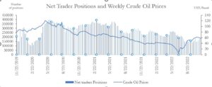
Figure 1: Correlation analysis between Net Commitment of Traders for Managed Money speculators and Crude Oil prices between 2019 and 2022

 

A correlation analysis

According to Figure 1 of this paper, the correlation between speculative positions and oil prices is 0.3878, indicating a moderate positive correlation between these two variables. This suggests some relationship between the amount of money being managed in crude oil markets and the prices of crude oil.

We conduct a correlogram (appendix 1) to explore the relationship between WTI further managed money positions and prices at different lags. We choose then the lag 7, as it will be detailed in the optimal lag choice in this paper’s second part, for weekly data.

In this correlogram, at lag 0, the correlation coefficient is 0.3878, indicating a positive relationship between Speculative Positions and Crude Oil Prices. The correlation coefficient gradually decreases as the lag increases indicating that the relationship between the two variables weakens as the time lag increases.

At lead 7, the correlation coefficient is 0.1481, indicating a weak positive relationship between the two variables. Overall, this correlogram suggests that there is a positive relationship between Speculative Positions and Crude Oil Prices, but the strength of the relationship weakens as the time lag increases.

For the positive lag, we conclude that managed money speculative positions in crude oil  leading crude oil prices. This is because the correlation between managed money and prices is positive at lag 0 and increases as the lag increases, while the correlation between prices and managed money is not significant at any lag. This suggests that changes in managed money in crude oil may be a leading indicator of changes in crude oil prices.

It’s important to note that correlation does not imply causation, so this negative correlation does not necessarily imply that WTI prices are causing changes in net positions or vice versa. In the second part of the paper, we will explore the relationship between these variables and BRENT and Volatility Index.

A market reading analysis.

From a market analysis point of view, crude oil price swings over the last three years allow us to understand commodities’ sensitivity to external shocks. Demand and Supply remain among the key factors contributing to the movement of commodities prices on financial markets. From a supply point of view, the non-OPEC supply growth was slower in 2019. An overall balance was maintained during the year, primarily due to the success of efforts coming from the countries participating in the Declaration of Cooperation (DoC). The speculative positions’ behavior in 2019 typically followed oil prices and shifts in demand levels, with upward and downward movements every week since November 2019.

On the other hand, 2020 started on a higher note for speculative positions, introduced by raising fears of the COVID-19 surge but also responding to demand and offer evolutions. Accordingly, in July 2020, the IEA produced an oil market report highlighting significant events occurring during the year’s first half. The fall in global demand and the oil supply decline were mainly discussed as the key drivers of the crude oil market. For the period ranging from April to June 2020, the speculative positions on crude oil prices were on a fast growth track. According to the IEA, lower demand volumes were recorded between April and June in that same context. Global oil production in June was around 13.7 mb/d, even lower than in April 2020.

Assuming that commitment of traders had a significant influence on the price movements, the price fluctuations are expected to move upward if traders’ speculative positions are higher than the previous week. The closing price is supposed to decrease if the speculative positions are lower than the last value.

In the period starting from the end of 2019 to 2022, the crude oil speculative positions did not move into a negative territory, which laid the ground for the constant interest of speculators in the crude oil market to maintain their positioning in positive territory even in periods of low prices, such as February 2020. A different scenario could be explored for the West Texas Intermediate prices, especially with negative territory prices in April 2020.

Moreover, in 2022, the oil industry experienced significant changes and developments. West Texas Intermediate (WTI) and Brent crude oil prices rose to $94 and $101 per barrel, respectively, marking an increase of 39% and 43% compared to the previous year. Russian oil exports to India reached a new high of 1.3 million barrels daily. The International Monetary Fund (IMF) predicted that global growth would slow down to 2.7% in the following year, with half of the European Union countries expected to experience a recession. China’s economy only grew by 3%, falling short of Beijing’s target of 5.5%. Non-OPEC supply was expected to expand by 1.5 million barrels per day, led by the United States, which was predicted to account for 75% of total growth. (Nakhle, 2023)

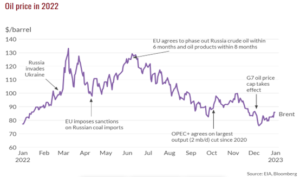
Figure 2: Crude Oil market movements in 2022

While speculative positions and crude oil prices seem to move to the same territory on a global scale, the econometric analysis provided in the following section will allow us to determine if this link instead stands solid between WTI prices and speculative positions and if the upward and downward movements are linked.

Furthermore, as observed in Figure 1 of this paper, correlation analysis does not allow drawing a direct and concrete link between speculation and prices for crude oil. Therefore, the second part of this paper will focus on an econometric study of the relationship between crude oil prices (both WTI and Brent) and provide further information about their relationship with increased volatility through the WTI speculative positions and the CBOE index for crude oil volatility. A Vector Autoregression Model, Granger Causality, and Fully Modified Least Squares model will be introduced to estimate the relationship between the abovementioned endogenous[8] variables.

1. An econometric exploration of the link between oil prices, volatility, and managed money investment

 Much of the research literature introduces the relationship between oil price  changes, oil shocks and long-term equilibrium positions between oil prices and product prices.  To complete the study of the correlation between commodities’ price movements and the positions taken by the managed money category of investors’ commitments of trading, the analysis of the causality test allows an understanding of which of the two abovementioned variables was able to exercise a higher pressure. This overall draws a broader understanding of how energy commodities, and oil specifically, respond to speculation, and to what extent non-commercial speculation leads to higher prices, based on the collected data movement between January 2010 and November 2022.

We focus on U.S. spot petroleum product prices. We utilize  Brent oil (FOB) spot prices as a first proxy for the global oil benchmark; we then complete it with WTI prices to have a full representation of Oil prices (Ederingtona et.al, 2020) We represent information based on spot prices for Brent and WTI oil prices, obtained from the archives of the U.S. Energy Information Administration (www.eia.gov). We chose not to remove seasonality, according to Beckers and Beidas-Storm’s work on forecasting the nominal brent oil price (Beckers and Beidas-Storm, 2015). Moreover, it appears that there is a lack of significant seasonal patterns in both WTI and Brent prices (see Figures 3 and 4 below).

Speculative positions are extracted, as mentioned above in this paper from the Weekly Net Commitment of Traders provided by CME group platform, representing the final commitment reported on Tuesday, highlighting the commitments undertaken by speculators between Monday and Friday of the previous week.

In this paper, we use the CBOE Crude Oil ETF Volatility Index (OVX) which is often compared to the implied volatility index (VIX), the trademark of Chicago board options exchange (CBOE), introduced in 1993, and further modified in 2003.

The CBOE Volatility Index is an up-to-the-minute market gauge that reflects anticipated volatility in the next 30 days.

The Chicago Board Options Exchange (CBOE) publishes the index and is commonly used by traders and investors to make informed decisions about crude oil-related investments. Investors commonly utilize the VIX to assess the degree of danger, apprehension, or pressure in the market while determining investment strategies. Similarly, to the VIX, the OVX measures market volatility, and reflects the volatility of different underlying assets. The OVX is a measure of the market’s expectation for the volatility of the United States Oil Fund, LP (USO), which is an Exchange-Traded Fund (ETF) that tracks the price of West Texas Intermediate (WTI) light, sweet crude oil. The OVX is calculated using the prices of certain options on the USO ETF and reflects the implied volatility of those options. In essence, the OVX provides investors with a measure of the expected level of volatility in the crude oil market over the next 30 days. It thus measures the expected volatility of crude oil prices.

Time Series Data:

We use weekly data from January 2010 to November 2022. The BRENT and WTI prices are extracted weekly from the EIA’s website. The weekly prices of Investors’ positions correspond to the difference between long and short commitment of traders weekly from the CME group’s website report for WTI positions as they provide a more extensive data sample compared to Brent prices. The OVX is used as a predictive tool for spot returns of WTI and Brent (Chen, et. Al, 2018). The weekly OVX returns are extracted from the FRED website and do not contain any seasonality. The weekly data provided for the OVX are aggregated in the Average method and are provided in Index units.

Abbreviation	Description	Source
Brent_prices	Weekly brent prices	www.eia.gov
Cboe_crude_oil_etf_volatility	Commodities volatility index	www.fred.saintlouisfed.org
WTI prices	Weekly WTI prices	www.eia.gov
Net_positions	Weekly Commitment of traders	www.cmegroup.com

 

Table 1: Description of the time series data

• Econometric data Methodology

1. Granger Causality

Granger causality analysis is a statistical approach that examines how information flows between time series (Stokes and Purdon, 2017).  Granger causality tests are a widely used statistical tool in econometrics, finance, and other fields to examine causal relationships between time-series variables. The tests were developed by Nobel laureate Clive Granger in the 1960s and are based on the principle that if one variable can be used to predict another variable, then the first variable is said to “Granger cause” the second variable.

We first conduct a stationarity test (appendix 3), then use the Granger Causality to examine the direction of causality by testing the reverse relationship.

However, it should be noted that Granger causality tests only identify statistical causality and do not necessarily imply a true causal relationship between the variables. Despite this limitation, Granger causality tests are a valuable tool for examining relationships between variables and can help  to inform policy decisions and investment strategies. In this paper, we use Granger causality tests to investigate the causal relationships between four macroeconomic variables and examine their implications for policy and investment decisions.

The use of Granger Causality in Oil studies has been widely reported, such as in the study of renewable energy, oil prices, and economic activity (Troster, et al., 2018), the study of real oil prices after the Great Recession (Benk and Gillman, 2017), or the causality investigation in high crude oil prices (Obadi, et al., 2013).

We witness there is evidence of causality in some cases, while in other cases, there is not enough evidence to reject the null hypothesis. Specifically, evidence suggests that the CBOE Crude Oil ETF Volatility Index Granger causes Brent Prices, but the relationship is not very strong.

On the other hand, Brent Prices Granger cause the CBOE Crude Oil ETF Volatility Index. There is also weak evidence to suggest that Net Positions Granger cause Brent Prices, but strong evidence suggests that Brent Prices Granger cause Net Positions.

There is no evidence to suggest that WTI Prices Granger cause Brent Prices or the CBOE Crude Oil ETF Volatility Index. However, strong evidence to suggest that the CBOE Crude Oil ETF Volatility Index Granger causes WTI Prices.

Additionally, there is weak evidence to suggest that WTI Prices Granger causes Net Positions, and that Net Positions Granger causes WTI Prices. Overall, the Granger causality test results suggest that there are causal relationships between some of the time series studied but not all.

Overall, the Granger causality test results indicate causal relationships between crude oil volatility, crude oil prices, and speculative activity in oil markets. However, the causal relationships are not universal, some are stronger than others. Specifically, there is evidence that the Crude Oil volatility Granger causes Brent Prices and WTI Prices, while Brent Prices Granger causes Crude Oil Volatility and Speculative Positions. There is weak evidence however, to suggest that Speculative Positions Granger causes Brent Prices and WTI Prices, and that WTI Prices Granger cause Net Positions. Nonetheless, the Granger causality test does not support the causal relationships between WTI Prices and Brent Prices.

In the same context, the findings of Obadi and Korcek (2018) suggest a bidirectional Granger Causality between oil price and investment positioning of money managers, suggesting that money managers are not only causing but also following oil price trends to make a profit and, in this way, they exaggerate the range of oil price moves.

In the case of our time series data and through the Granger Causality test, it seems that we can only confirm the latter relationship of money managers following oil price trends, which eventually leads into profit making, as suggested by a part of the literature around commodities’ financialization.

1. Vector Autoregression

Vector Autoregression Model

Vector Autoregression (VAR) models are a class of time-series models that allow for the analysis of multiple interrelated variables. VAR models are used to model the joint dynamics of two or more time-series variables, allowing for the estimation of causal relationships and predicting future values. VAR models do not impose a structural form on the model, unlike Structural VAR models. Instead, they assume that each variable in the system is affected by its own past values and the past values of the other variables in the system.

Since the 1980s, Christopher Sims provided a new macro-econometric framework that held great promise: vector autoregressions (VARs). A univariate autoregression is a single-equation, single-variable linear model in which the current value of a variable is explained by its lagged values. VAR models describe the joint generation process of a few variables over time, so they can be used for investigating relationships between the variables. Granger causality is one type of relationship between time series (Granger, 1969).

We chose here to employ the VAR models to study, through the corresponding lags, the extent of the impact of some endogenous variables on one another.

The residual Cholesky figures in appendices 6, 7, and 8 of this paper are used to analyse the causal relationships among variables and to gain insights into the underlying dynamics of the system being modelled, examining the Cholesky residual graph, we can identify the strength and direction of the causal relationships among the variables in the VAR model.

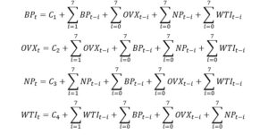
Suppose the 4 endogenous variables introduced in our paper. Let’s name them the following:

 

 

BP: Brent Prices

OVX: Crude Oil Volatility ETF Index

NP : Net Positions

WTI: WTI Prices

We set up a VAR model to describe the relationship between our four endogenous variables. We have used the VAR methodology to find the relationship between the four-time series and the optimal lag of 7 as identified above.

Our 4 equations for the VAR model are then the following:

Cholesky Impulse Responses

Case 1: Impulse Responses to Changes in Net Positions

In the Impulse Response Functions highlighted in Appendix 7, we have highlighted the answer of Brent Prices to a one standard deviation shock in Net Positions, the answer of OVX (Crude Oil Volatility Index) to a one Standard Deviation shock in Net Positions and finally the answer of WTI Prices to a one standard deviation shock in Net Positions.

The Volatility Index starts with a timid response to Net Positions and then decreases through a sharp decline over time. The Brent prices’ answer to one Standard Deviation Change in WTI Managed Positions suggests a gradual increase in Brent Prices reactions, that reach a maximum level period eight on the Cholesky Impulse Response graph. A similar response is observed in WTI prices, with a gradual increase between periods 0 and 10, and a maximum level reached in the eighth period. These answers suggest that investors in the answer in WTI and Brent prices are following the same pattern regarding reactions to investors positions.

It has been proved in the literature that WTI and Brent’s prices are highly positively correlated, with a value of 0.8285, according to the findings of Zhang (2022). On the other hand, a lead-lag relationship has also been explored between WTI and Brent prices, suggesting that WTI spot prices lead the Brent spot prices, on a low level. (Yang, et. Al, 2020). In our time series data, we find that the WTI response is slightly higher than the one of BRENT in the first period. This could be explained by the direct impact of investors’ positions on WTI itself rather than BRENT, or as suggested by the literature, by the leading relationship between WTI and Brent.

Case 2: Impulse Responses to Changes in WTI Prices

According to the Impulse Response Functions in appendix 8, we have highlighted the answer of Net Positions to a one standard deviation shock in WTI Prices, the answer of OVX (Crude Oil Volatility Index) to a one Standard Deviation shock in WTI Prices.

Accordingly, the Net Positions’ answer to one Standard Deviation change in WTI prices, suggests a sharp increase in the first period. The pattern is then(?) rather decreasing from periods two to three, then another increase is observed from the third to fourth periods. A sharp decrease is the observed between the fifth and seventh periods, to finally a convergence to 0 between eighth and ninth periods.

These findings suggest that WTI prices significantly impact both Net Positions and crude oil volatility, and that the relationship between these variables is complex and dynamic over time.

Case 3: Impulse Responses to changes in OVX (Crude Oil Volatility Index)

The relationship between WTI prices and the OVX index, as observed through the Cholesky Impulse Response Functions in Appendix 9, indicates that a one standard deviation shock in OVX index causes a shift in the dynamic of WTI prices. Specifically, the response of WTI prices to a shock in OVX index is observed to be increasing from periods one to three, followed by a decrease from period three to five. However, a sharp increase is then noticed between periods seven to ten. These findings suggest the OVX index has a significant impact on the behavior of WTI prices, with changes in crude oil volatility leading to shifts in the dynamics of the WTI market.

Following the responses of case 2 and the ones of case 3, we can assume that the relationship between WTI and OVX is bidirectional, with a change in WTI prices impacting the OVX index, and vice versa. An increase or decrease in WTI prices could affect crude oil’s volatility, which would then be reflected in the OVX index. Similarly, a shock in OVX index could impact the behavior of WTI prices, as observed through the Cholesky Impulse Response Functions discussed earlier. Overall, the relationship between WTI and OVX is complex and dynamic, with changes in one variable potentially impacting the behavior of the other.

The Brent Prices response to one standard deviation shock in OVX index is declining from 0 to 6, with it failing to return to a positive territory. However, a sharp increase is noticed between periods 6 to 10 with a shift to positive territory starting period. This suggests that there could be a lagged response of Brent Prices to changes in crude oil volatility, with market participants adjusting their positions over time in response to changes in OVX. Overall, the relationship between OVX and Brent Prices is complex and dynamic, with changes in one variable potentially impacting the behavior of the other over time.

Finally, the Net Positions response to the OVX index also starts on a negative territory. Between periods 0 to 4, it fails to exceed 0 and goes on positive territories. Between periods 5 to 7, it increases sharply, then falls slightly between 6 and 7 to rise again starting period 8. The highest increase is; however the one noticed between periods 5 to 7. The sharp increase in the net positions between periods 5 to 7 could indicate that there was a positive trend in the market during that period. Overall, we consider that there is an inverse relationship between the OVX index and net positions, meaning that when the OVX index increases, the net positions decrease and vice versa.

In summary, the Cholesky Impulse Response Functions analysis suggests complex and dynamic relationships exist between Brent prices, WTI prices, OVX (Crude Oil Volatility Index), and Net Positions. Changes in one variable can impact the behavior of the others over time, and the relationships between variables can be bidirectional.

In Case 1, the response of Brent prices, WTI prices, and OVX to changes in Net Positions suggest that investors in WTI and Brent prices follow similar patterns in reactions to investors’ positions, with a slight lead of WTI prices.

In Case 2, the response of Net Positions and OVX to changes in WTI prices suggests that WTI prices have a significant impact on both variables, and the relationship between these variables is complex and dynamic over time.

In Case 3, the response of WTI prices, Brent prices, and Net Positions to changes in OVX suggests that changes in crude oil volatility can impact the behavior of these variables, with the relationships between variables being complex and dynamic over time.

These findings highlight the importance of considering the dynamic relationships between variables in the crude oil market when making investment decisions.

1. Fully Modified Least Squares

Phillips and Hansen introduced the Fully Modified Least Squares (FM-OLS) regression technique to obtain optimal estimates of cointegrating regressions. The method adjusts least squares to consider the serial correlation effects and the endogeneity in the regressors, which result from the existence of a cointegrating relationship (Phillips, 1995).

The Fully Modified Least Squares (FMOLS) is a regression method used in econometrics to estimate the long-run relationship between variables. It is commonly used when there is a possibility of endogeneity and when the analyzed variables are non-stationary.

The output of a FMOLS regression provides estimates of the long-run coefficients for the independent variables and their t-statistics and probabilities. In addition, the method provides a long-run covariance estimate and the long-run variance of the dependent variable. FMOLS is a useful tool for analyzing the long-run relationship between variables and providing insights into their potential causal links.

The results of the FMOLS show the output of a Fully Modified Least Squares (FMOLS) analysis with the dependent variable being NET_POSITIONS. The model estimates the long-run relationship between the dependent variable our pendent variables: OVX, BRENT_PRICES, WTI_PRICES, and C (a constant term).

The FMOLS analysis tests for cointegration, which implies the existence of a long-run relationship between the variables. The cointegrating equation in this analysis includes a constant term. The coefficient estimates for the four independent variables are presented in the table. OVX has a negative coefficient, indicating that an increase in OVX is associated with a decrease in NET_POSITIONS in the long run. BRENT_PRICES also has a negative coefficient, but it is not statistically significant at the 5% level. WTI_PRICES has a positive coefficient, but it is also not statistically significant at the 5% level. Finally, the constant term has a positive coefficient, indicating that on average, NET_POSITIONS tend to be positive.

The R-squared value is 0.064489, indicating that the model explains a relatively small proportion of the variation in the dependent variable. The adjusted R-squared value is slightly lower, indicating that the including of the independent variables may not be improving the model significantly. The standard error of the regression is 87621.55, representing the average distance the data points fall from the fitted line. The long-run variance estimate is also presented, which is a measure of the volatility of NET_POSITIONS over the long run.

The econometric models employed to analyze further  the relationship between the commitment of managed money traders, the prices of crude oil, and the OVX as an indicator of volatility confirm the complex relationship between movements in oil markets and the behavior of investors. Accepting or refuting the argument of the managed money positions contribute to price volatility remains a complex subject where one good answer cannot be provided.

Parameters such as the studied periods, inherent oil shocks, and the relationship with exogenous variables such as the impact of the USD on crude oil can provide further information related to this topic. However, it remains key to recall another time, the  importance, and the relevancy of the movement in fundamental markets that contribute highly to shifting the investors’ sentiment, and the prices on the markets.

1. Conclusion, discussions, and recommendations

Conclusion

The financialization of commodities has brought both positive and negative implications. While it has increased liquidity and facilitated hedging activities, one could argue that it has also led to increased volatility in commodity markets, which can have negative impacts on producers and consumers.

The role of speculators in commodity markets can also be controversial, as they may disrupt the equilibrium of the markets and generate price movements that do not reflect the underlying supply and demand conditions. It is crucial to consider the different motivations and behaviors of market participants, including hedgers, speculators, and traders, to understand the dynamics of commodity markets and their implications for the broader economy.

In that context, the use of data and analysis, such as the CFTC’s weekly reports on speculative positions, can provide valuable insights into the short-term movements of commodity markets and help to inform decision-making by market participants and policymakers.

Based on the results presented, this study examined the causal relationships and long-run dynamics between crude oil prices, investor positions, and volatility using weekly data from January 2010 to November 2022. The Brent and WTI prices, as well as investor positions, were extracted from the EIA and CME Group’s websites, respectively. The OVX was used as a predictive tool for spot returns of WTI and Brent, and its weekly returns were extracted from the FRED website.

The Granger causality tests showed that there is weak evidence to suggest that Net Positions cause a movement in WTI and Brent prices. However, strong evidence suggests that Brent and WTI prices Granger cause net positions. There is also evidence to suggest that the CBOE Crude Oil ETF Volatility Index Granger causes Brent prices, but the relationship is not very strong, and Brent prices Granger cause the CBOE Crude Oil ETF Volatility Index.

The findings of Obadi and Korcek (2018) support a bidirectional Granger causality between oil prices and investment positioning of money managers, suggesting that money managers are not only causing but also following oil price trends to make a profit and exaggerating the range of oil price moves.

The VAR model outputs, suggest the complex and dynamic relationships between our four variables, with changes in one variable impacting the behavior of the others over time. The relationship between these variables is bidirectional, with changes in one variable impacting the other, and vice versa. Overall, the analysis highlights the significant impact of WTI prices on both Net Positions and crude oil volatility, and the complex and dynamic relationship between WTI prices and the OVX index.

The Fully Modified Least Squares (FMOLS) analysis tested for cointegration, which implies the existence of a long-run relationship between our variables. The constant term has a positive coefficient, indicating that on average, net positions tend to be positive on average. OVX has a negative coefficient, indicating that an increase in OVX is associated with a decrease in net positions in the long run.

Overall, the results suggest that there are significant causal relationships and long-run dynamics between crude oil prices, investor positions, and volatility. The findings have important implications for investors, policymakers, and market participants in understanding the factors that influence crude oil prices and the behavior of market participants in the oil market. Further research may be required to investigate the complex interactions between these variables and their impact on the global economy.

Future Directions

In conclusion, this study has highlighted the positive and negative implications of the financialization of commodities, with a specific focus on crude oil markets. The findings suggest that while financialization has increased liquidity and facilitated hedging activities, it has also led to increased volatility in commodity markets, which can have negative impacts on producers and consumers. The role of speculators in commodity markets is also controversial and requires further investigation to understand the dynamics of commodity markets and their implications for the broader economy.

Moreover, the results have shown significant causal relationships and long-run dynamics between crude oil prices, investor positions, and volatility. Future research could focus on improving the model by using alternative methodologies or testing for different variables. Additionally, researchers may consider expanding the study to include other commodities or examining the impact of geopolitical events on commodity markets. These analyses could provide valuable insights into the behavior of market participants and inform decision-making by market participants and policymakers.

Policy recommendations

The energy market has witnessed the financialization of commodities, which has resulted in both positive and negative outcomes. On the one hand, it has augmented liquidity and facilitated hedging activities. On the other hand, it has also caused increased volatility in commodity markets, potentially harming producers and consumers. In addition, the involvement of speculators in commodity markets could generate significant controversy, as it could disturb the equilibrium of the markets and cause price fluctuations that are not aligned with the fundamental supply and demand conditions.

To address these issues, policymakers in the energy market may consider implementing regulations that limit excessive speculation and promote transparency in commodity markets. Additionally, they may consider measures to promote the development of physical markets for energy commodities, which can provide greater price stability and reduce the impact of financial speculation on energy prices. In the short term, policymakers may use data and analysis, such as the CFTC’s weekly reports on speculative positions, to monitor market trends and inform decision-making by market participants and policymakers.

In the long term, policymakers may consider promoting renewable energy technologies and investing in infrastructure to support the transition to a low-carbon economy. This can reduce reliance on fossil fuels and decrease the susceptibility of energy markets to price volatility. Additionally, policies promoting energy efficiency and conservation can reduce demand for energy commodities and decrease the impact of financial speculation on energy prices. Overall, these policy recommendations can help to promote a more stable and sustainable energy market.

Acknowledgments

We would like to express our sincere gratitude to Yves Jégourel for his guidance and support throughout the writing of this paper. His insights, feedback, and suggestions were instrumental in shaping our research and improving the quality of our analysis.

 

 

1. References

Al-Zoghivy and Tayachi, 2021, Saudi Stock Market, Energy prices and gold prices: an empirical study of their dynamic relationship, 2021.

Bal and Dash, 2020, Nonlinear Granger causality between oil price and stock returns in India, Wiley Online Libreray, https://onlinelibrary.wiley.com/doi/abs/10.1002/pa.2137

Bahattin Büyükşahin, Jeffrey H. Harris, 2011, Do Speculators Drive Crude Oil Futures Prices? The Energy Journal, Vol. 32, No. 2 (2011), pp. 167-202 (36 pages) https://www.jstor.org/stable/41323326

Basak and Pavlova, 2016, A Model of Financialization of Commodities, The Journal of Finance, https://onlinelibrary.wiley.com/doi/abs/10.1111/jofi.12408

 

Bhayani, R., “Crude Oil Speculative Positions Rise Sharply Following Price Fall.” www.business-standard.com, November 26, 2018, https://www.business-standard.com/article/economy-policy/crude-oil-speculative-positions-rise-sharply-following-price-fall-118112600921_1.html

Becker and Beidas-Strom, 2015, Forecasting the Nominal Brent Oil Price with VARs-One Model Fits All?, IMF e-libreary, https://www.elibrary.imf.org/view/journals/001/2015/251/article-A001-en.xml

Bonato, M., Taschini, L., “Comovement and Financialization in the Commodity Market.” SSRN Electronic Journal, 2015. https://doi.org/10.2139/ssrn.2573551

Chen, et. Al, 2018, The predictive content of CBOE crude oil volatility index, Elsevier, https://www.sciencedirect.com/science/article/abs/pii/S0378437117310865

Cheng, H., Xiong, W., “Financialization of Commodity Markets.” Annual Review of Financial Economics, December 1^st, 2014, https://doi.org/10.1146/annurev-financial-110613-034432

CFTC, 2023, https://www.cftc.gov/LearnAndProtect/EducationCenter/CFTCGlossary/glossary_m.html

Chiappini & Jégourel, 2019, Explaining the role of commodity traders: A theoretical approach, Economics Bulletin, https://ideas.repec.org/a/ebl/ecbull/eb-18-00771.html

Ding, et. Al, 2021, The effects of commodity financialization on commodity market volatility, https://www.sciencedirect.com/science/article/abs/pii/S0301420721002312

Ederingtona, et.Al, 2021, The relation between petroleum product prices and crude oil prices, Elsevier, https://www.sciencedirect.com/science/article/pii/S0140988320304199

Federal Reserve Bank of Chicago, (2017), “Financialization in Commodity Markets – Federal Reserve Bank of Chicago,” https://www.chicagofed.org/publications/working-papers/2017/wp2017-15

Financial Stability Review, 2011, The Macrofinancial Environment, https://www.ecb.europa.eu/pub/financialstability/fsr/focus/2011/pdf/ecb~6fdfdfce1c.fsrbox201112_04.pdf

Granger, 1969, Investigating Causal Relations by Econometric Models and Cross-spectral Methods, August 1969, https://www.jstor.org/stable/1912791

Goldstein, et. Al, 2014, Speculation and Hedging in Segmented Market, Oxford Journals, https://www.jstor.org/stable/pdf/24465696.pdf?refreqid=excelsior%3Abfaa4b498cf98263be27e6bd0c82918e&ab_segments=&origin=&initiator=

Kang, et.Al, 2013, The Role of Hedgers and Speculators in Liquidity Provision to Commodity Futures Markets https://conference.nber.org/confer/2013/CWf13/Kang_Rouwenhorst_Tang.pdf

Kuffman, et.Al, 2009, Oil prices, speculation, and fundamentals: Interpreting causal relations among spot and futures prices, International Labour Organization, https://labourdiscovery.ilo.org/discovery/fulldisplay?docid=cdi_gale_infotracacademiconefile_A200850790&context=PC&vid=41ILO_INST:41ILO_V1&lang=en&search_scope=MyInst_and_CI&adaptor=Primo%20Central&tab=Everything&query=sub,exact,%20Prices%20,AND&mode=advanced&offset=30

Ludwing, 2019, Speculation and its impact on liquidity in commodity markets, https://ideas.repec.org/a/eee/jrpoli/v61y2019icp532-547.html

Liu, et. Al, 2011, The Price Correlation between Crude Oil Spot and Futures –Evidence from Rank Test, https://www.sciencedirect.com/science/article/pii/S187661021101112X

Nakhle, 2023, Oil markets: An early peek into 2023, https://www.gisreportsonline.com/r/oil-2023/

Newbery, 1987, When Do Futures Destabilize Spot Prices?, Wiley, https://www.jstor.org/stable/pdf/2526724.pdf?refreqid=excelsior%3A470250cd43cf5f871c9db970b1850d51&ab_segments=&origin=&initiator=

Nicolau, et. Al, 2013, “Are Futures Prices Influenced by Spot Prices or Vice-versa? An Analysis of Crude Oil, Natural Gas and Gold Markets”, Universita Politecnica delle Marche, http://docs.dises.univpm.it/web/quaderni/pdf/394.pdf

Obadi and Korcek, 2018, The Crude Oil Price and Speculations: Investigation Using
Granger Causality Test, International Journal of Energy Economics and Policy?, ISSN: 2146-4553 www.econjournals.com

Obadi, et. Al, 2013, “What are the Causes of High Crude Oil Price? Causality Investigation.” www.ecojournals.com, https://dergipark.org.tr/en/download/article-file/361266

Philipps, 1995, Fully Modified Least Squares and Vector Autoregression, Econometrica, Vol. 63, No. 5 (Sep., 1995), pp. 1023-1078 (56 pages), https://www.jstor.org/stable/2171721

Shabbir, et.Al, 2020, Impact of gold and oil prices on the Stock Market in Pakistan, Journal of Economics, Finance and Administrative Science, http://www.scielo.org.pe/scielo.php?pid=S207718862020000200279&script=sci_arttext&tlng=pt

Szilard and Gillman, 2017, “Granger-causality of real oil prices after the Great Recession”, December 28th, 2017

Troster, , et. Al, 2013, “Renewable energy, oil prices, and economic activity: A Granger-causality in quantiles analysis”, February 2019 https://www.sciencedirect.com/science/article/pii/S0140988318300379

 

World Bank Group, 2023, “Commodity Markets: Evolution, Challenges, and Policies.” World Bank, January 3^rd, 2023. https://www.worldbank.org/en/research/publication/commodity-markets

1. Appendices and Econometrics Methodology

 

Date: 04/06/23   Time: 15:33
Sample: 11/22/2019 12/09/2022
Included observations: 155
Correlations are asymptotically consistent approximations
CRUDE_OIL_MANAGED_MONEY, CRUDE_OIL_PRICES(-i)	CRUDE_OIL_MANAGED_MONEY, CRUDE_OIL_PRICES(+i)	i	lag	lead
. |****     |	. |****     |	0	0.3878	0.3878
. |****     |	. |***      |	1	0.4231	0.3473
. |*****    |	. |***      |	2	0.4573	0.3106
. |*****    |	. |***      |	3	0.4812	0.2685
. |*****    |	. |**       |	4	0.5018	0.2348
. |*****    |	. |**       |	5	0.5258	0.2040
. |*****    |	. |**       |	6	0.5378	0.1733
. |*****    |	. |*.       |	7	0.5484	0.1481

Appendix 1: Cross Correlogram of Crude_Oil_Managed_Money and Crude_Oil_Prices

	Mean	Std. Dev.	Maximum	Minimum	Skewness	Kurtosis
BRENT_PRICES	7.751.278	2.666.949	1.274.000	1.424.000	0.081011	1.814.589
CBOE_CRUDE_OIL_ETF_VOLATILITY_INDEX_	3.728.258	1.775.589	2.345.220	1.522.000	4.744.727	4.024.818
NET_POSITIONS	221918.0	109180.5	1720512.	-311783.0	3.952.922	5.531.744
WTI_PRICES	7.114.126	2.292.752	1.204.300	3.320.000	0.001428	1.894.996

 

Appendix 2: Descriptive Statistics

1. Stationarity of data

We first test for the presence of unit roots in the oil price, net positions and volatility index price series in logarithm. Unit root tests are conducted to ensure that all variables are in a stationary form. A stationary data is one that does not show any trend, as non-stationary data cannot provide valid results, which is why many researchers do not accept it. Stationarity is key in time series analysis because it allows for the use of certain statistical models and techniques that assume that the data is stationary. Non-stationary time series can lead to biased results and incorrect conclusions. Therefore, unit root tests are essential in determining the stationarity of a time series and in selecting appropriate statistical models for analysis.

The Augmented Dickey-Fuller test can be used to check the stationary of data. This test checks for the unit root hypothesis, which assumes that the time collection has a unit base. If the data is non-stationary, it may result in a loss of power. The unit root test focuses on the time collection rather than the range of observation. This test is applied to all variables at the level and on the first difference. In this study, a decision was made at a 0.05% level of significance, and all variables were in a stationary format on first difference. (Shabbir, et. Al, 2020). The ADF tests for the four variables are available in appendix 1 of this paper.

In this time series, the stationarity of Brent Oil Prices and WTI Oil Prices is only ensured at the first difference levels. Whereas for the Net Positions and the OVX, the ADF shows the stationarity of data without referring to first and second differences. On the other hand, the ADF test shows the message exogenous: constant for both WTI Oil Prices and Brent Oil Prices. When running an ADF test with exogenous variables, implying that the ADF test was run with a constant term as an exogenous variable.

The constant term in the ADF test represents the long run mean of the time series and assumes that the series has a constant trend over time. By including the constant term as an exogenous variable, the ADF test is able to determine whether the time series is stationary around a constant trend.

Null Hypothesis: D(WTI_PRICES) has a unit root
Exogenous: Constant
Lag Length: 0 (Automatic – based on SIC, maxlag=54)
			t-Statistic	Prob.*
Augmented Dickey-Fuller test statistic			-2.264.713	0.0000
Test critical values:	1% level		-3.439.925
	5% level		-2.865.656
	10% level		-2.569.019
*MacKinnon (1996) one-sided p-values.

 

 

Null Hypothesis: D(BRENT_PRICES) has a unit root
Exogenous: Constant
Lag Length: 0 (Automatic – based on SIC, maxlag=53)
			t-Statistic	Prob.*
Augmented Dickey-Fuller test statistic			-21.68889	0.0000
Test critical values:	1% level		-3.439925
	5% level		-2.865656
	10% level		-2.569019
*MacKinnon (1996) one-sided p-values.

 

Null Hypothesis: D(CBOE_CRUDE_OIL_ETF_VOLATILITY_INDEX__INDEX__WEEKLY__NOT_SEASONALLY_ADJUSTED) has a unit root
Exogenous: None
Lag Length: 1 (Automatic – based on SIC, maxlag=53)
			t-Statistic	Prob.*
Augmented Dickey-Fuller test statistic			-21.52783	0.0000
Test critical values:	1% level		-2.568439
	5% level		-1.941299
	10% level		-1.616380
*MacKinnon (1996) one-sided p-values.

 

 

Null Hypothesis: D(NET_POSITIONS) has a unit root
Exogenous: None
Lag Length: 4 (Automatic – based on SIC, maxlag=53)
			t-Statistic	Prob.*
Augmented Dickey-Fuller test statistic			-17.08237	0.0000
Test critical values:	1% level		-2.568455
	5% level		-1.941301
	10% level		-1.616378
*MacKinnon (1996) one-sided p-values.

 

Appendix 3: ADF tests

1. Selection of optimum lag length

The study of optimum lag length is a prerequisite to conduct the econometric models selected. The lag-lengths selected on the basis of Akaike information criteria (AIC), Schwarz information criteria (SIC) or Hannan-Quinn information and the Final Prediction Error as suggested by the work of Al-Zoghiby and Tayachi (2021) in their work on the Saudi Stock Market, energy prices and gold prices.

In selecting the optimal lag for weekly Brent Prices, WTI prices, Net Positions and CBOE Crude Oil prices, we retain the lags in rank 7 estimated at 38.03713, 6.15e+11 and 38.49671 in Likelihood Ratio (LR), Final Prediction Error (FPE) and Akaike Information Criterion respectively.

 

Lag	LogL	LR	FPE	AIC	SC	HQ
0	-16273.98	NA	2.89e+16	49.25259	49.27979	49.26313
1	-12739.80	7014.896	6.87e+11	38.60757	38.74353*	38.66026
2	-12688.74	100.7298	6.18e+11	38.50148	38.74623	38.59634*
3	-12680.50	16.16468	6.33e+11	38.52495	38.87847	38.66197
4	-12659.41	41.08104	6.23e+11	38.50957	38.97186	38.68874
5	-12643.79	30.25932	6.24e+11	38.51070	39.08177	38.73204
6	-12627.05	32.19839	6.23e+11	38.50849	39.18833	38.77198
7	-12607.16	38.03713*	6.15e+11*	38.49671*	39.28533	38.80236
8	-12601.13	11.46602	6.34e+11	38.52687	39.42426	38.87468
* indicates lag order selected by the criterion
LR: sequential modified LR test statistic (each test at 5% level)
FPE: Final prediction error
AIC: Akaike information criterion
SC: Schwarz information criterion
HQ: Hannan-Quinn information criterion

 

Appendix 4: VAR lag-length selection criteria

 

1. Granger Causality Test

 

Pairwise Granger Causality Tests
Date: 04/01/23   Time: 14:12
Sample: 1/12/2010 11/15/2022
Lags: 7
Null Hypothesis:	Obs	F-Statistic	Prob.
CBOE_CRUDE_OIL_ETF_VOLATILITY_INDEX__INDEX__ WEEKLY__NOT_SEASONALLY_ADJUSTED does not Granger Cause BRENT_PRICES	662	1.97097	0.0567
BRENT_PRICES does not Granger Cause CBOE_CRUDE_OIL_ETF_VOLATILITY_ INDEX__INDEX __WEEKLY__NOT_SEASONALLY_ADJUSTED		3.69040	0.0006
NET_POSITIONS does not Granger Cause BRENT_PRICES	662	1.99614	0.0534
BRENT_PRICES does not Granger Cause NET_POSITIONS		2.78463	0.0074
WTI_PRICES does not Granger Cause BRENT_PRICES	662	0.58190	0.7710
BRENT_PRICES does not Granger Cause WTI_PRICES		1.66936	0.1136
NET_POSITIONS does not Granger Cause CBOE_CRUDE_OIL_ETF_VOLATILITY_INDEX__INDEX__WEEKLY__ NOT_SEASONALLY_ADJUSTED	662	0.88998	0.5139
CBOE_CRUDE_OIL_ETF_VOLATILITY_INDEX__INDEX__WEEKLY__ NOT_SEASONALLY_ADJUSTED does not Granger Cause NET_POSITIONS		1.98256	0.0552
WTI_PRICES does not Granger Cause CBOE_CRUDE_OIL_ETF_VOLATILITY_INDEX__INDEX__WEEKLY__ NOT_SEASONALLY_ADJUSTED	662	3.00042	0.0042
CBOE_CRUDE_OIL_ETF_VOLATILITY_INDEX__INDEX__WEEKLY__ NOT_SEASONALLY_ADJUSTED does not Granger Cause WTI_PRICES		2.16874	0.0352
WTI_PRICES does not Granger Cause NET_POSITIONS	662	4.38441	9.E-05
NET_POSITIONS does not Granger Cause WTI_PRICES		3.44028	0.0013

 

Appendix 5: Granger Causality Analysis

Based on the Granger causality test results in appendix 1, representing our time series, we can conclude that there is evidence of causality in some cases, while in other cases, there is not enough evidence to reject the null hypothesis that one time series does not Granger cause the other. Specifically, we can conclude that there is evidence to suggest that the CBOE Crude Oil ETF Volatility Index does Granger cause Brent Prices, but the relationship is not very strong (F-Statistic = 1.97097, p-value = 0.0567). On the other hand, Brent Prices Granger causes the CBOE Crude Oil ETF Volatility Index (F-Statistic = 3.69040, p-value = 0.0006).

Moreover, there is weak evidence to suggest that Net Positions Granger cause Brent Prices (F-Statistic = 1.99614, p-value = 0.0534). However, there is strong evidence to suggest that Brent Prices Granger cause Net Positions (F-Statistic = 2.78463, p-value = 0.0074).

There is no evidence to suggest that WTI Prices Granger cause Brent Prices, and vice versa (both p-values > 0.05). There is no evidence to suggest that Net Positions Granger cause the CBOE Crude Oil ETF Volatility Index, and vice versa (both p-values > 0.05). Similarly, to Brent prices, is strong evidence to suggest that the CBOE Crude Oil ETF Volatility Index Granger cause WTI Prices (F-Statistic = 3.00042, p-value = 0.0042). There is weak evidence to suggest that WTI Prices Granger cause Net Positions (F-Statistic = 4.38441, p-value = 9.E-05), and that Net Positions Granger cause WTI Prices (F-Statistic = 3.44028, p-value = 0.0013).

1. VAR Model Estimates

 

	BRENT_PRICES	NET_POSITIONS	OVX	WTI_PRICES
BRENT_PRICES(-1)	1.129421	-827.7220	-0.328527	0.109239
	(0.08233)	(898.993)	(0.20467)	(0.08053)
	[ 13.7175]	[-0.92072]	[-1.60517]	[ 1.35652]
BRENT_PRICES(-2)	-0.137043	1235.603	0.439978	-0.040667
	(0.11942)	(1303.92)	(0.29685)	(0.11680)
	[-1.14758]	[ 0.94761]	[ 1.48214]	[-0.34817]
BRENT_PRICES(-3)	0.131596	-1245.461	-1.109545	0.045487
	(0.11963)	(1306.22)	(0.29738)	(0.11701)
	[ 1.10002]	[-0.95348]	[-3.73109]	[ 0.38875]
BRENT_PRICES(-4)	-0.219611	1107.941	1.854506	-0.216078
	(0.12093)	(1320.43)	(0.30061)	(0.11828)
	[-1.81599]	[ 0.83908]	[ 6.16907]	[-1.82684]
BRENT_PRICES(-5)	0.086128	-167.5462	-1.010233	0.148061
	(0.12429)	(1357.14)	(0.30897)	(0.12157)
	[ 0.69294]	[-0.12346]	[-3.26967]	[ 1.21793]
BRENT_PRICES(-6)	-0.001012	344.0555	-0.434334	0.097137
	(0.12344)	(1347.77)	(0.30684)	(0.12073)
	[-0.00820]	[ 0.25528]	[-1.41551]	[ 0.80459]
BRENT_PRICES(-7)	-0.010942	-414.3879	0.556448	-0.121849
	(0.08195)	(894.746)	(0.20370)	(0.08015)
	[-0.13352]	[-0.46313]	[ 2.73169]	[-1.52030]
NET_POSITIONS(-1)	1.05E-05	0.795517	-7.39E-06	1.63E-05
	(3.7E-06)	(0.04088)	(9.3E-06)	(3.7E-06)
	[ 2.79880]	[ 19.4615]	[-0.79418]	[ 4.44025]
NET_POSITIONS(-2)	-6.15E-06	0.141497	-6.96E-06	-1.01E-05
	(4.7E-06)	(0.05184)	(1.2E-05)	(4.6E-06)
	[-1.29643]	[ 2.72973]	[-0.58995]	[-2.17880]
NET_POSITIONS(-3)	-5.47E-06	-0.031560	6.35E-06	-6.66E-06
	(4.8E-06)	(0.05256)	(1.2E-05)	(4.7E-06)
	[-1.13655]	[-0.60041]	[ 0.53043]	[-1.41503]
NET_POSITIONS(-4)	8.85E-06	-0.030766	-5.41E-06	5.91E-06
	(4.8E-06)	(0.05257)	(1.2E-05)	(4.7E-06)
	[ 1.83819]	[-0.58525]	[-0.45174]	[ 1.25566]
NET_POSITIONS(-5)	-1.14E-06	0.049499	1.10E-05	-2.95E-07
	(4.8E-06)	(0.05273)	(1.2E-05)	(4.7E-06)
	[-0.23596]	[ 0.93873]	[ 0.91310]	[-0.06250]
NET_POSITIONS(-6)	-4.89E-06	0.028288	-7.33E-06	-4.01E-06
	(4.8E-06)	(0.05200)	(1.2E-05)	(4.7E-06)
	[-1.02669]	[ 0.54404]	[-0.61918]	[-0.86176]
NET_POSITIONS(-7)	-1.24E-06	-0.007044	4.55E-06	1.41E-07
	(3.7E-06)	(0.04094)	(9.3E-06)	(3.7E-06)
	[-0.32983]	[-0.17208]	[ 0.48837]	[ 0.03845]
OVX(-1)	-0.023931	37.95698	0.838332	0.017095
	(0.01806)	(197.227)	(0.04490)	(0.01767)
	[-1.32488]	[ 0.19245]	[ 18.6706]	[ 0.96764]
OVX(-2)	0.031021	-67.60411	-0.047327	-0.003342
	(0.02441)	(266.498)	(0.06067)	(0.02387)
	[ 1.27096]	[-0.25368]	[-0.78005]	[-0.14001]
OVX(-3)	-0.007002	149.3535	0.198637	-0.005614
	(0.02426)	(264.893)	(0.06031)	(0.02373)
	[-0.28863]	[ 0.56383]	[ 3.29379]	[-0.23659]
OVX(-4)	-0.015245	-19.81903	-0.128198	-0.013510
	(0.02395)	(261.504)	(0.05953)	(0.02342)
	[-0.63653]	[-0.07579]	[-2.15333]	[-0.57676]
OVX(-5)	-0.004229	132.4326	0.206126	-0.022669
	(0.02372)	(259.041)	(0.05897)	(0.02320)
	[-0.17825]	[ 0.51124]	[ 3.49520]	[-0.97693]
OVX(-6)	0.052784	63.45900	-0.057622	0.033045
	(0.02384)	(260.359)	(0.05927)	(0.02332)
	[ 2.21364]	[ 0.24374]	[-0.97213]	[ 1.41689]
OVX(-7)	-0.020052	-208.4234	-0.129203	0.013070
	(0.01791)	(195.544)	(0.04452)	(0.01752)
	[-1.11966]	[-1.06586]	[-2.90225]	[ 0.74617]
WTI_PRICES(-1)	-0.015551	2677.987	-0.029212	0.991555
	(0.09013)	(984.098)	(0.22404)	(0.08815)
	[-0.17255]	[ 2.72126]	[-0.13039]	[ 11.2482]
WTI_PRICES(-2)	0.027496	-2686.610	-0.109400	-0.081054
	(0.12757)	(1392.89)	(0.31711)	(0.12477)
	[ 0.21554]	[-1.92881]	[-0.34499]	[-0.64963]
WTI_PRICES(-3)	-0.049265	1139.019	1.260931	0.051091
	(0.12827)	(1400.50)	(0.31884)	(0.12545)
	[-0.38409]	[ 0.81329]	[ 3.95471]	[ 0.40725]
WTI_PRICES(-4)	0.002214	-1694.172	-1.982317	0.047703
	(0.13076)	(1427.70)	(0.32503)	(0.12789)
	[ 0.01693]	[-1.18665]	[-6.09879]	[ 0.37300]
WTI_PRICES(-5)	0.053188	-190.5685	1.116690	-0.070694
	(0.13469)	(1470.60)	(0.33480)	(0.13173)
	[ 0.39491]	[-0.12959]	[ 3.33537]	[-0.53665]
WTI_PRICES(-6)	0.116725	-0.109169	0.204830	0.000108
	(0.13451)	(1468.73)	(0.33438)	(0.13156)
	[ 0.86776]	[-7.4e-05]	[ 0.61258]	[ 0.00082]
WTI_PRICES(-7)	-0.113212	635.9933	-0.450033	0.034268
	(0.09136)	(997.562)	(0.22711)	(0.08936)
	[-1.23916]	[ 0.63755]	[-1.98158]	[ 0.38349]
C	-0.438798	14737.23	7.267241	-0.665730
	(0.72548)	(7921.40)	(1.80341)	(0.70957)
	[-0.60484]	[ 1.86043]	[ 4.02972]	[-0.93822]
R-squared	0.989259	0.887241	0.850221	0.986090
Adj. R-squared	0.988783	0.882254	0.843596	0.985475
Sum sq. resids	5102.213	6.08E+11	31527.91	4880.867
S.E. equation	2.839079	30999.35	7.057416	2.776813
F-statistic	2082.072	177.8843	128.3297	1602.658
Log likelihood	-1615.294	-7770.730	-2218.110	-1600.613
Akaike AIC	4.967654	23.56414	6.788853	4.923303
Schwarz SC	5.164577	23.76106	6.985776	5.120225
Mean dependent	77.54707	221099.0	37.31682	71.08302
S.D. dependent	26.80703	90339.74	17.84521	23.04024
Determinant resid covariance (dof adj.)		5.16E+11
Determinant resid covariance		4.31E+11
Log likelihood		-12624.62
Akaike information criterion		38.49131
Schwarz criterion		39.27900
Number of coefficients		116

Appendix 6: VAR Estimates Table

The VAR model includes four variables: BRENT_PRICES, NET_POSITIONS, OVX, and WTI_PRICES and includes lagged values of each variable as predictors. The coefficients for each variable at different lags are given in the table. The coefficients indicate the change in each variable that is associated with a one-unit change in the lagged variable, holding all other variables constant. The numbers in parentheses below the coefficients are the standard errors.

The numbers in square brackets are t-statistics, which measure the number of standard errors by which the estimated coefficient differs from zero. A t-statistic greater than 2 (or less than -2) suggests that the coefficient is statistically significant at the 5% level.

For example, looking at the first row, we can see that a one-unit increase in the lagged value of BRENT_PRICES (BRENT_PRICES(-1)) is associated with a 1.13 unit increase in BRENT_PRICES, on average, holding all other variables constant. This coefficient is statistically significant at the 5% level, with a t-statistic of 13.72.

1. VAR model output: Cholesky One Standard Deviation Impulse responses

Appendix 7: Impulse Responses to changes in Net Positions

Appendix 8: Impulse Responses to changes in WTI prices

Appendix 9: Impulse Responses to changes in OVX Index

1. Fully Modified Least Square

Dependent Variable: NET_POSITIONS
Method: Fully Modified Least Squares (FMOLS)
Date: 04/01/23   Time: 15:41
Sample (adjusted): 1/19/2010 11/01/2022
Included observations: 668 after adjustments
Cointegrating equation deterministics: C
Long-run covariance estimate (Bartlett kernel, Newey-West fixed
bandwidth = 7.0000)
Variable	Coefficient	Std. Error	t-Statistic	Prob.
OVX	-953.5438	501.1281	-1.902794	0.0575
BRENT_PRICES	-2735.418	1508.305	-1.813570	0.0702
WTI_PRICES	2515.848	1776.347	1.416305	0.1572
C	288613.3	40887.59	7.058701	0.0000
R-squared	0.064489	Mean dependent var		220270.3
Adjusted R-squared	0.060262	S.D. dependent var		90387.32
S.E. of regression	87621.55	Sum squared resid		5.10E+12
Long-run variance	4.28E+10

Appendix 10: Fully Modified Least Square Model

 

[1] Economist at the Policy Center for the New South working on Energy and Commodities research.

[2] Senior Fellow at the Policy Center for the New South, principal at Center for Macroeconomics and Development and non-resident fellow at Brookings Institute. Former Vice President and Executive Director at the World Bank, Executive Director at the International Monetary Fund (IMF) and Vice President at the Inter-American Development Bank. He was also Deputy Minister for international affairs at Brazil’s Ministry of Finance, as well as professor of economics at University of São Paulo (USP) and University of Campinas (UNICAMP).

[3] Hedging activity can be undertaken for risk mitigation. This risk can be referred to as physical, financial or counterparty risk. By hedging we refer to investors willing to take positions for purposes other and not limited to speculating on commodities markets. However, as it is difficult to distinguish on a surface level which investors are entering long and short positions for adding liquidity to markets, hedging against a real risk, or for speculative purposes only, in this paper, speculators or hedgers, are assumed not to be linked to a pure speculative purpose, given the choice of the Managed Money Positions category on the CME group platform that will be detailed in this paper.

[4] The commodities’ settlement can both be achieved via Cash Settlement and Physical Delivery. While Cash Settlement mainly refers to a cash payment made by the purchaser or contract holders to execute the commodity settlement, the physical delivery refers to the literal delivery of underlying assets on the date of settlement. The physical delivery is generally insured by the clearing broker, or agent.

[5] The demand and offer are the primary price regulators for commodities if financial markets are not considered. However, the recent findings show an extension of price setters of commodities to external shocks, correlation with certain currencies such as the case of oil and USD and the interdependency between certain commodities’ prices from several categories. While the assessment of whether commodities financialization has been accountable for the spillover of external factors for the definition of commodities prices, it is first essential to focus on the organization of commodities’ financial markets, as well as to assess the behavior of commodities on financial exchange places, in the times of utmost sensitivity to exogenous political and economic factors, as well as solid market activity from non-commercial speculators.

[6] According to the Commodity Futures Trading Commission, the categories of participants include Managed Money Traders, as participants that engage in futures trades on behalf of investment funds or clients.

https://www.cftc.gov/LearnAndProtect/EducationCenter/CFTCGlossary/glossary_m.html#:~:text=Managed%20Money%20Trader%20(MMT)%3A,as%20well%20as%20hedge%20funds.

[7] Open Interest is defined as the total number of futures contracts held by market participants at the end of each trading date. It can be used as an indicator to determine market sentiment and the relevance of price trends. https://www.cmegroup.com/education/courses/introduction-to-futures/open-interest.html

[8] The 4 variables selected are influenced by various internal factors such as market fundamentals, supply and demand dynamics, market sentiment, and the actions of market participants such as traders, investors, and speculators which sustains their consideration as endogenous variables.